scTenifoldNet

scTenifoldNet is an R package for constructing and comparing single-cell gene regulatory networks (scGRNs) from single-cell RNA-seq (scRNA-seq) data collected under different conditions. It employs a machine-learning workflow combining principal component regression, tensor decomposition, and manifold alignment to accurately identify even subtly shifted gene expression programs.

Implementations in other languages are also available:

Python: scTenifoldpy
MATLAB: scGEAToolbox

Installation

scTenifoldNet is available on CRAN:

install.packages("scTenifoldNet")

To install the development version from GitHub:

# install.packages("remotes")
remotes::install_github("cailab-tamu/scTenifoldNet")

The package is written in R only, so installing from source needs no compiler.

Pipeline Overview

The scTenifoldNet() function orchestrates a six-step pipeline. Each step reports progress to the console via the cli package, with sample-level labels ([X] / [Y]) so that operations on each condition are clearly distinguishable.

Step	Function	Description
1	`scQC`	Quality control — filters cells by library size, outlier detection, minimum gene expression fraction, and mitochondrial read ratio
2	`cpmNormalization`	Counts-per-million (CPM) normalization
3	`makeNetworks`	Constructs gene regulatory networks from subsampled cells using principal component regression (`pcNet`). All the per-gene regressions come from one eigendecomposition, which gives the same networks as fitting each gene separately
4	`tensorDecomposition`	CANDECOMP/PARAFAC (CP) tensor decomposition for network denoising
5	`manifoldAlignment`	Non-linear manifold alignment of the two denoised networks
6	`dRegulation`	Differential regulation testing via Box-Cox transformation and chi-square statistics

Individual functions are exported and fully documented, allowing users to run or modify any step independently.

Input

The required input is a raw counts matrix with genes as rows and cells (barcodes) as columns. Data should be unnormalized when using the main scTenifoldNet() function. The modular design of the package allows users to substitute custom preprocessing at any step.

Output

scTenifoldNet() returns a list with three elements:

tensorNetworks — Weight-averaged denoised gene regulatory networks after CP tensor decomposition, containing:
- X: The network for sample X (sparse matrix of class dgCMatrix).
- Y: The network for sample Y (sparse matrix of class dgCMatrix).
The diagonal (self-loops) of both networks is set to zero. The CP decomposition can produce non-zero values there, but they are not used by the manifold alignment.
manifoldAlignment — A data frame of low-dimensional features from the non-linear manifold alignment, with 2 × n genes rows and d columns (default d = 30).
diffRegulation — A data frame with six columns:
- gene: Gene identifier.
- distance: Euclidean distance between the gene’s coordinates in the two conditions.
- Z: Z-score after Box-Cox power transformation.
- FC: Fold change with respect to the expectation.
- p.value: P-value from the chi-square distribution with one degree of freedom.
- p.adj: Adjusted p-value (Benjamini & Hochberg FDR correction).

Reproducibility

Network construction subsamples cells at random, so results depend on the random seed. The seed argument (default 1) is set before each random step. The same input and parameters therefore give the same result on every run, whatever the caller’s RNG state, and that state is restored when the function returns.

Use different values (seed = 1, seed = 2, …) to see how much results vary between runs.
Use seed = NULL to let a set.seed() call made before the function control the result.

tensorDecomposition() accepts the same seed argument.

Running Time

Running time grows mainly with the number of genes. The number of cells matters little, because each network is built from a fixed-size subsample of cells (nc_nCells). Benchmarks with the default parameters (10 networks of 500 cells) on simulated counts, measured on an Apple M2 Pro (16 GB RAM) with R 4.5 and its reference BLAS:

Cells	Genes	Time
300	1,000	35 s
1,000	1,000	33 s
1,000	5,000	8.4 min
2,500	5,000	7.9 min
5,000	5,000	8.0 min

Before version 1.4.1, networks were built by fitting one SVD per gene, and the earlier benchmarks in this README (measured on a different machine) reported about 3 hours for 5,000 genes.

Memory

Peak memory grows with the square of the number of genes, because the networks are stacked into a tensor of genes x genes x nc_nNet entries. Estimated peak memory with 10 networks:

Genes	Peak memory
1,000	0.8 GB
2,000	2.2 GB
5,000	11.8 GB
10,000	46 GB
15,000	103 GB

scTenifoldNet() compares this estimate with the memory available after quality control and warns, before building the networks, when it does not fit, reporting the largest number of genes that does. The estimate can also be checked beforehand with scTenifoldNet::checkMemory(nGenes, nNet = 10, nConditions = 2).

Example

Simulating a dataset

We create a sparse count matrix of 2,000 cells and 100 genes drawn from a negative binomial distribution (~67 % zeros). The last ten genes are prefixed with mt- to simulate mitochondrial genes.

library(scTenifoldNet)

nCells <- 2000
nGenes <- 100
set.seed(1)
X <- matrix(
  rnbinom(n = nGenes * nCells, size = 20, prob = 0.98),
  ncol = nCells
)
rownames(X) <- c(paste0("ng", 1:90), paste0("mt-", 1:10))

Generating a perturbed condition

Genes 10, 2, and 3 are replaced with the expression profiles of genes 50, 11, and 5, respectively.

Y <- X
Y[10, ] <- Y[50, ]
Y[2, ]  <- Y[11, ]
Y[3, ]  <- Y[5, ]

Running the pipeline

Under H₀ (no differential regulation) we supply the same matrix for both conditions. Under H_A we supply the control and perturbed matrices.

outputH0 <- scTenifoldNet(X = X, Y = X,
                          nc_nNet = 10, nc_nCells = 500,
                          td_K = 3, qc_minLibSize = 30)

outputHA <- scTenifoldNet(X = X, Y = Y,
                          nc_nNet = 10, nc_nCells = 500,
                          td_K = 3, qc_minLibSize = 30)

Inspecting the tensor networks

The denoised networks are stored as sparse matrices that can be converted to igraph objects for downstream topological analysis:

igraph::graph_from_adjacency_matrix(outputHA$tensorNetworks$X, weighted = TRUE)
igraph::graph_from_adjacency_matrix(outputHA$tensorNetworks$Y, weighted = TRUE)

Differential regulation results

Under H₀, no genes reach significance (FDR < 0.1). Under H_A, the six genes involved in the perturbation are correctly identified:

head(outputH0$diffRegulation, n = 6)
#    gene     distance        Z       FC    p.value     p.adj
# 59 ng59 1.138659e-15 2.497859 4.338493 0.03725989 0.6411916
# 32 ng32 9.970451e-16 2.081719 3.326448 0.06817394 0.6411916
# 72 ng72 9.452170e-16 1.917581 2.989608 0.08380044 0.6411916
# 89 ng89 8.924023e-16 1.742758 2.664849 0.10258758 0.6411916
# 12 ng12 8.851226e-16 1.718018 2.621550 0.10542145 0.6411916
# 17 ng17 8.784453e-16 1.695183 2.582145 0.10807510 0.6411916

head(outputHA$diffRegulation, n = 6)
#    gene   distance        Z        FC      p.value      p.adj
# 2   ng2 0.023526702 2.762449 12.193413 0.0004795855 0.02414332
# 50 ng50 0.023514429 2.761550 12.180695 0.0004828665 0.02414332
# 11 ng11 0.022443941 2.681598 11.096894 0.0008647241 0.02882414
# 3   ng3 0.020263415 2.508478  9.045415 0.0026335445 0.06583861
# 10 ng10 0.019194561 2.417929  8.116328 0.0043868326 0.07711821
# 5   ng5 0.019079975 2.407977  8.019712 0.0046270923 0.07711821

Visualizing the results

Quantile-quantile plots provide a clear summary. Genes with FDR < 0.1 are highlighted in red.

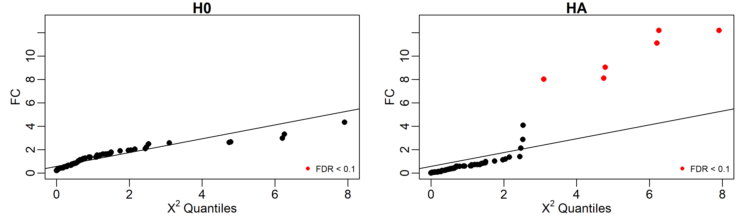
par(mfrow = c(2, 1), mar = c(3, 3, 1, 1), mgp = c(1.5, 0.5, 0))
set.seed(1)
qChisq <- rchisq(100, 1)

geneColor <- rev(ifelse(outputH0$diffRegulation$p.adj < 0.1, "red", "black"))
qqplot(qChisq, outputH0$diffRegulation$FC, pch = 16, main = expression(H[0]),
       col = geneColor, xlab = expression(chi^2 ~ Quantiles), ylab = "FC",
       xlim = c(0, 8), ylim = c(0, 13))
qqline(qChisq)
legend("bottomright", legend = "FDR < 0.1", pch = 16, col = "red", bty = "n", cex = 0.7)

geneColor <- rev(ifelse(outputHA$diffRegulation$p.adj < 0.1, "red", "black"))
qqplot(qChisq, outputHA$diffRegulation$FC, pch = 16, main = expression(H[A]),
       col = geneColor, xlab = expression(chi^2 ~ Quantiles), ylab = "FC",
       xlim = c(0, 8), ylim = c(0, 13))
qqline(qChisq)
legend("bottomright", legend = "FDR < 0.1", pch = 16, col = "red", bty = "n", cex = 0.7)

Citation

If you use scTenifoldNet in your research, please cite:

Osorio, D., Zhong, Y., Li, G., Huang, J. Z., & Cai, J. J. (2020). scTenifoldNet: A Machine Learning Workflow for Constructing and Comparing Transcriptome-wide Gene Regulatory Networks from Single-Cell Data. Patterns, 1(9), 100139. doi:10.1016/j.patter.2020.100139

BibTeX:

@Article{osorio2020sctenifoldnet,
  title   = {scTenifoldNet: A Machine Learning Workflow for Constructing and
             Comparing Transcriptome-wide Gene Regulatory Networks from
             Single-Cell Data},
  author  = {Daniel Osorio and Yan Zhong and Guanxun Li and Jianhua Z. Huang
             and James J. Cai},
  journal = {Patterns},
  year    = {2020},
  volume  = {1},
  number  = {9},
  pages   = {100139},
  issn    = {2666-3899},
  doi     = {10.1016/j.patter.2020.100139},
}