hexify

Hexagonal Grids for Global Spatial Analysis — ISEA + H3

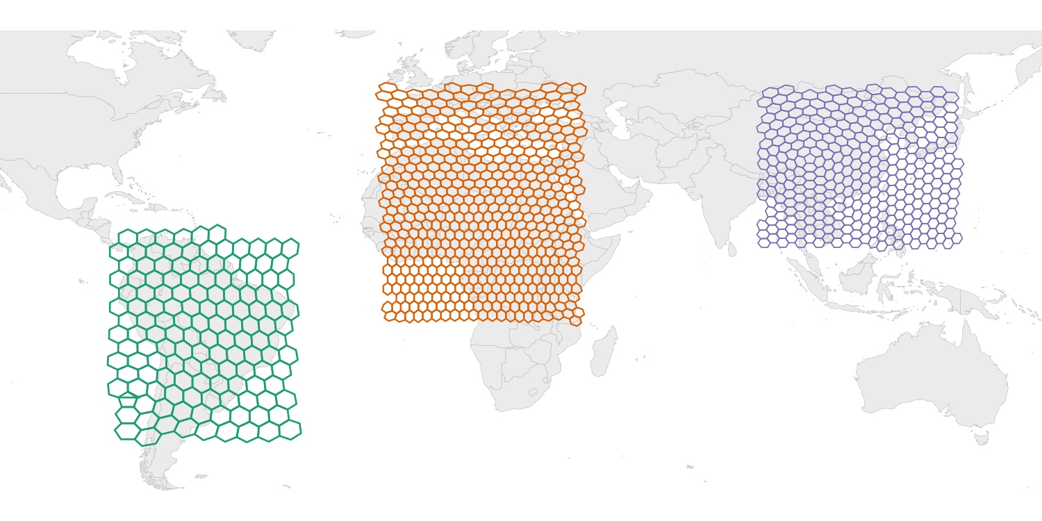
The hexify package provides fast, accurate assignment of geographic coordinates to hexagonal grid cells. It supports two grid systems: ISEA (Icosahedral Snyder Equal Area) for guaranteed equal-area cells, and H3 (Uber’s hierarchical hex system) for compatibility with industry-standard workflows like FCC broadband mapping. Whether you’re aggregating species occurrences, analyzing point patterns, or preparing data for spatial modeling, hexify gives you one consistent interface for both systems.

Quick Start

library(hexify)

cities <- data.frame(
  name = c("Vienna", "Paris", "Madrid"),
  lon = c(16.37, 2.35, -3.70),
  lat = c(48.21, 48.86, 40.42)
)

# ISEA equal-area grid (default)
grid <- hex_grid(area_km2 = 10000)
result <- hexify(cities, lon = "lon", lat = "lat", grid = grid)
plot(result)

# H3 grid (Uber's system)
h3_grid <- hex_grid(resolution = 4, type = "h3")
result_h3 <- hexify(cities, lon = "lon", lat = "lat", grid = h3_grid)
plot(result_h3)

Statement of Need

Spatial binning is fundamental to ecological modeling, epidemiology, and geographic analysis. Standard approaches using rectangular lat-lon grids introduce severe area distortions: a 1° cell at the equator covers ~12,300 km², while the same cell near the poles covers a fraction of that area. This violates the equal-sampling assumption underlying most spatial statistics.

Discrete Global Grid Systems (DGGS) solve this by partitioning Earth’s surface into cells of uniform area. hexify implements two hex grid systems:

• ISEA — True equal-area hexagonal grids with apertures 3, 4, 7, or mixed 4/3. Fast C++ implementation. Compatible with dggridR cell IDs.
• H3 — Uber’s hierarchical hexagonal system (resolutions 0–15). Industry standard used by the FCC, Foursquare, and others. Powered by the h3o package.

Both systems share the same interface: hexify(), cell_to_sf(), grid_rect(), get_parent(), get_children(), and all other functions work with either grid type.

These features make hexify suitable for:

• Species distribution modeling and biodiversity assessments
• Epidemiological surveillance and disease mapping
• Environmental monitoring and remote sensing aggregation
• Any analysis requiring unbiased spatial binning

Features

Core Workflow

• hex_grid(): Define a grid by target cell area (km²) or resolution level
• hexify(): Assign points to grid cells (data.frame or sf input)
• plot() / hexify_heatmap(): Visualize results with base R or ggplot2

Grid Generation

• grid_rect(): Generate cell polygons for a bounding box
• grid_global(): Generate a complete global grid (all cells)
• grid_clip(): Clip grid to a polygon boundary (country, region, etc.)

Cell Operations

• cell_to_sf(): Convert cell IDs to sf polygon geometries
• cell_to_lonlat(): Get cell center coordinates
• get_parent() / get_children(): Navigate grid hierarchy

Interoperability

• as_dggrid() / from_dggrid(): Convert to/from dggridR format
• as_sf(): Export HexData to sf object
• as.data.frame(): Extract data with cell assignments
• H3 support: hex_grid(resolution = 8, type = "h3") — requires h3o package

Installation

# Install from CRAN
install.packages("hexify")

# Or install development version from GitHub
# install.packages("pak")
pak::pak("gcol33/hexify")

Usage Examples

Basic Point Assignment

library(hexify)

# Define grid: ~10,000 km² cells
grid <- hex_grid(area_km2 = 10000)
grid
#> HexGridInfo: aperture=3, resolution=5, area=12364.17 km²

# Assign coordinates to cells
coords <- data.frame(
  lon = c(-122.4, 2.35, 139.7),
  lat = c(37.8, 48.9, 35.7)
)
result <- hexify(coords, lon = "lon", lat = "lat", grid = grid)

# Access cell IDs
result@cell_id

Working with sf Objects

library(sf)

# Any CRS works - hexify transforms automatically
points_sf <- st_as_sf(coords, coords = c("lon", "lat"), crs = 4326)
result <- hexify(points_sf, area_km2 = 10000)

# Export back to sf
result_sf <- as_sf(result)

Generating Grid Polygons

# Grid for Europe
grid <- hex_grid(area_km2 = 50000)
europe_hexes <- grid_rect(c(-10, 35, 40, 70), grid)
plot(europe_hexes["cell_id"])

# Clip to a country boundary
library(rnaturalearth)
france <- ne_countries(country = "France", returnclass = "sf")
france_grid <- grid_clip(france, grid)

Aggregating Point Data

# Species occurrence data
occurrences <- data.frame(
  species = sample(c("Sp A", "Sp B", "Sp C"), 1000, replace = TRUE),
  lon = runif(1000, -10, 30),
  lat = runif(1000, 35, 60)
)

# Assign to grid
grid <- hex_grid(area_km2 = 20000)
occ_hex <- hexify(occurrences, lon = "lon", lat = "lat", grid = grid)

# Count per cell
occ_df <- as.data.frame(occ_hex)
occ_df$cell_id <- occ_hex@cell_id

cell_counts <- aggregate(species ~ cell_id, data = occ_df, FUN = length)
names(cell_counts)[2] <- "n_records"

# Richness per cell
richness <- aggregate(species ~ cell_id, data = occ_df,
                      FUN = function(x) length(unique(x)))
names(richness)[2] <- "n_species"

Visualization

# Quick plot
plot(result)

# Heatmap with basemap
hexify_heatmap(occ_hex, value = "n_records", basemap = TRUE)

# Custom ggplot
library(ggplot2)
cell_polys <- cell_to_sf(cell_counts$cell_id, grid)
cell_polys <- merge(cell_polys, cell_counts, by = "cell_id")

ggplot(cell_polys) +
  geom_sf(aes(fill = n_records), color = "white", linewidth = 0.2) +
  scale_fill_viridis_c() +
  theme_minimal()

Documentation

• Quick Start - Basic concepts and workflow
• Visualization - Plotting with base R and ggplot2
• Workflows - Grid generation, clipping, multi-resolution analysis

Support

“Software is like sex: it’s better when it’s free.” — Linus Torvalds

I’m a PhD student who builds R packages in my free time because I believe good tools should be free and open. I started these projects for my own work and figured others might find them useful too.

If this package saved you some time, buying me a coffee is a nice way to say thanks. It helps with my coffee addiction.

Citation

@software{hexify,
  author = {Colling, Gilles},
  title = {hexify: Equal-Area Hexagonal Grids for Spatial Analysis},
  year = {2025},
  url = {https://CRAN.R-project.org/package=hexify},
  doi = {10.32614/CRAN.package.hexify}
}

License

MIT (see LICENSE.md)